Can BM25 be a probability?

We’ve built on a BM25 foundation. These unbounded lexical relevance scores could be 0.51, 5.6, or 12.21. It’s often said you can’t interpret them, don’t even try. Just sort on them.

But other relevance factors? Could easily be modeled as probabilities: embedding similarities, click thru rate, page rank, recency, conversion rates and so on.

Because these can be made probabilities, combining their scores can be rigorously grounded. Probabilities can be ‘AND’d” and “OR’d”. We can score by treating the simpler factors as priors.

But not lexical scores. Those seem all over the place.

For historical reasons, we gave BM25 primacy. We don’t question the decades of development, inherited through Lucene, where BM25 came first. Everything else must be layered on top.

Because of this, we now live in a world that assumes:

• We’ll get a BM25 score to start with
• We can manipulate it up and down with additive boosts
• We play with these magic numbers game until ranking conforms to what we expect

If we want to merge with other systems (like embeddings) we don’t dare try to combine the underlying factors. We get by with interleaving their rankings with Reciprocal Rank Fusion.

Hybrid search practitioners struggle, not because of embeddings, but because BM25 fails to fit into clean expectations of a probability.

Somebody took a principled look at this problem: Bayesian BM25. Today’s a bit of a review of BB25. You’ll see it creates a framework for BM25 to be turned into a probability. From there we might think about hybrid search from first principles differently.

BM25: probabilistic but not a probability

Why are BM25 scores so weird?

One reason, ironically, is BM25’s foundation in probabilistic Information Retrieval. BM25 models odds* not probabilities.

Lexical search measures: “if we see a term match, does that mean its relevant (R=1) or irrelevant (R=0)?”

rel_odds(t) = P(t|R=1) / P(t|R=0)

To build this model, it’s most useful to think about the denominator:

Why would a term match occur in an irrelevant doc? We can think of a few reasons:

• Maybe the user searched a common and ambiguous term (searching a movie website for ‘luke’ could match many things unrelated to the user’s intent).
• Maybe the term matched a spurious mention (the term ‘skywalker’ mentioned once in a book doesn’t mean its a book about Star Wars).

We don’t need to belabor the excellent writing out there on BM25. BM25 models these odds with term frequency (more occurrences, better), field length (matches in shorter docs better), and a term’s doc frequency (lower better)

BM25’s creates a statistic for ranking term matches. It just needed to be sortable, descending. It didn’t anticipate being combined with other factors - and definitely not embeddings. BM25 WAS relevance in its creators estimation.

It was Judge Dredd. I AM THE LAW!

While it thinks its the law - its the odd one out. BB25 tries to fix that.

BB25 - Bayesian BM25 → better hybrid search

Can bring BM25 back into the world of probabilities?

That’s what Bayesian BM25 attempts to do. (notebook here)

In Bayesian BM25, we compute a probability from two factors:

• A prior - default assumption of relevance for a query in a doc, before seeing a BM25 score
• A likelihood - how likely we would see this evidence (a BM25 score) for a relevant (or irrelevant) doc?

If you’re new to Bayesian thinking, an example might be helpful.

Say we believe a sports team has a low probability of winning the championship. They’ve performed poorly all season. That’s our prior.

Then a game is played. It’s a great game! The team wins. Set aside the teams record for now - How likely would this win be for a championship team? For a last place team?

That’s the likelihood - how likely this evidence, a game score, occurs for the possible scenarios (championship team or not).

Now, we’ll be slightly less pessimistic about the team. Still pessimistic, but able to see a glimmer of hope. We call our updated belief the posterior 🍑.

That’s what BB25 does with search.

• BB25 starts with a lexical prior with simple term statistics. That’s our baseline assumption of relevance.
• Then it uses the BM25 score as evidence, the game that was just played,
• Then it computes likelihood: compatibility between the belief “this is a relevant doc” and “we observed this BM25 score”,
• Then, using an actual dataset, it fits this whole process so that probabilities produced from BB25 correspond to ground truth labels (more on this is a sec)

That’s the theory at least. As we walk through the BB25 implementation, you might quibble with details. But I hope you feel inspired to experiment.

BB25 Prior

The BB25 prior uses two factors

• Term frequency - more terms, a higher prior
• Field norms - shorter docs, a higher prior

Let’s quickly look at the term frequency prior:

tf_prior = 0.2 + 0.7 * min(1, TERM_FREQ / 10)

We take term frequency, divide it by 10. When TF crosses 10, the highest this it won’t contribute further (the min(...) forces this to 1). tf_prior can be at minimum 0.2, at most 0.9.

The norm prior has a similar pattern. Any document more than half the average doc length we return 0.3 + 0.6 * (0.5) or 0.6. Anything shorter we might return 0.6 to 0.9.

bm25_norm_length = LENGTH / AVG_DL
norm_prior = 0.3 + 0.6 * (1 - min(bm25_norm_length, 0.5))

We combine these into the final prior, weighing TF higher than norms.

bb25_prior = clamp(0.7 * tf_prior + 0.3 * norm_prior,
                   0.1,
                   0.9)

There’s plenty to quibble with, and probably could be improved. Like other scoring system, we’ve found a heuristic that seems to work for the author. But probably not nearly as battle tested as the original BM25 scoring (remember its the 25th iteration!).

The prior also doesn’t care about document frequency. The prior for 3 occurrences of “the” in a doc would be the same as 3 occurrences of “polyvagal”. No consideration yet for term specificity Since IDF lives in the the likelihood, the next term we’ll discuss, we don’t need to worry just yet.

So I bet someone else could come up with perhaps a better formulation. But for now, we should be impressed that Bayesian BM25 is forcing us to rethink BM25 to be a probability.

BB25 likelihood - BM25 scaled

In Bayesian statistics, the likelihood moves away from the prior to update our belief.

Here we pass the BM25 score passed through a sigmoid to scale it from 0-1. Close to 1: this BM25 score we expect a championship team / relevant doc. And vice versa.

The parameters of this likelihood

• Alpha, steepness - how quickly the function transitions from 0 → 1. The authors start with 1.
• Beta, the midpoint - the BM25 score above which 50% more relevant. The authors suggest starting with the median BM25 score

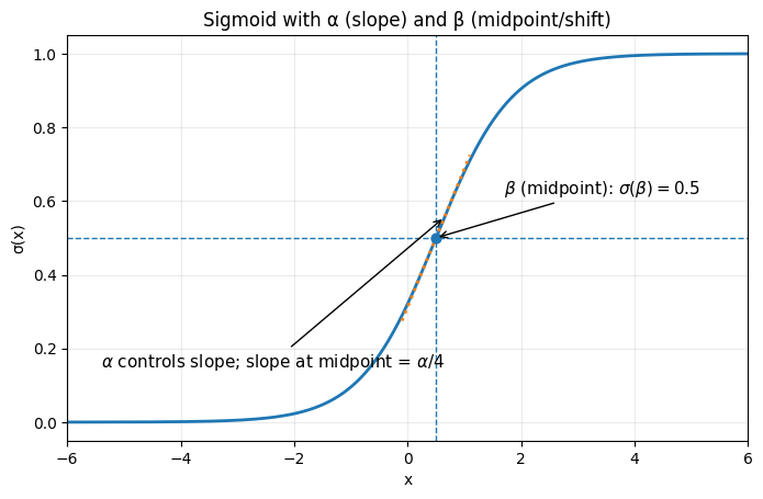
More precisely, the likelihood is:

def sigmoid(x: float) -> float:
    """
    Numerically stable sigmoid function.

    σ(x) = 1 / (1 + e^-x)
    """
    if x >= 0:
        z = math.exp(-x)
        return 1 / (1 + z)
    else:
        z = math.exp(x)
        return z / (1 + z)

bb25_likelihood = sigmoid(ALPHA * (bm25_score - BETA))

Now we might critique a few things

Particularly: we have to find BETA - the median BM25 score of the corpus. This requires calibration / learning on a specific dataset against labels. More on this in a minute.

The final BB25 probability

Finally we combine these through using Bayes Theorem.

bb25_lp = bb25_prior * bb25_likelihood
bb25_marginal = bb25_lp + (1 - bb25_likelihood) * (1 - bb25_prior)
bb25_posterior = bb25_lp / bb25_marginal

Calibration of probability

The real power of Bayesian BM25 comes in its calibration step. While we might quibble with the prior and likelihood, the ability to learn their parameters from labels makes the probabilities sensible + usable downstream.

Why do we need calibrated probabilities? Why not just use this to scale probabilities?

We need calibrated probabilities for hybrid search to make sense. Consider a probabilistic AND between the probability of relevance, given an embedding P(R | E) and the probability of relevance given a lexical score P(R | L)

P(R | E) * P(R | L)

They may not be calibrated against each other. An embedding similarity for one query may simply be larger, dominating the final score. A max lexical probability of 0.5 puts the lexical score at a disadvantage against embedding similarities.

So the paper uses gradient descent, against labels, to optimize alpha / beta for the BM25 side (presumably we could do this for the embedding side). In the linked notebook, I show calibration for the Wayfair WANDS dataset on the product_name field’s BM25 score:

iterations = 50
learning_rate = 0.01
num_samples = 10000
alpha = 1
beta = bm25_judgments['score'].median()

for idx in range(iterations):
    alpha_grad = 0; beta_grad = 0;
    for index, row in bm25_judgments.sample(num_samples, random_state=idx).iterrows():
       
        # Scale this examples BM25 score
        bm25_score = row['score']
        pred = sigmoid(alpha * (bm25_score - beta))
   
		    # Compute error (label - pred)
        label = row['grade']
        error = label - pred
        
        # Update our gradient for alpha / beta given
        # this error
        alpha_grad += error * bm25_score
        beta_grad += -error * alpha
        
    # Actually update alpha / beta
    alpha -= learning_rate * alpha_grad / num_samples
    beta -= learning_rate * beta_grad / num_samples
    print(alpha, beta)

# Compute a calibrated score
bm25_judgments['score_calibrated'] = bm25_judgments.apply(lambda row: sigmoid(alpha * (row['score'] - beta)), axis=1)

Now the most relevant docs have score_calibrated close to 0.99, and least relevant close to 0.15.

Critiques and other approaches

As I’ve been writing this post, I’ve heard different philosophies on combining probabilistic evidence of relevance. For example, another perspective exists in this paper from Craswell et. al. While the paper discusses query independent evidence (ie document page rank, etc), it provides a philosophy worth considering

• BM25 is already probabilistic, but its a likelihood ratio P(t|R=1) / P(t|R=0)
• We shouldn’t try to force BM25 to be a probability
• We should provide tools to make other factors look like BM25 (scaling with log, saturation, etc)

You can see this approach realized in the rank feature query in Elasticsearch.

Even here, calibrating BM25 against other evidence takes work. Often we’re playing with different boosts, etc to achieve this.

Just learn the boosts

On the other hand, there’s a different philosophy: Just learn the boosts™️. Notably, everything I’ve done above is on a single field. That’s not practical. Usually we’re working across many lexical fields.

What I’ve taught in the past for hybrid search:

• Embedding score E
• Lexical BM25 score L

Assume you want an “AND” like formulation:

S = (e*E) * (l*L) # AND lexical / embedding
S = (e*E) + (l+L) # "OR" lexical / embedding
...

You literally can learn lexical weight l, embedding weight e through random search (ie trying random values and picking the best). It’s underrated and very practical. If you want to get fancier you can do Bayesian optimization on the params (a different notion of Bayes).

You’re not calibrating trying to create good probabilities. Here L / E live on different scales. So you’re just picking magic numbers that predict the final score. What you lose: interpretability of these intermediate factors. If they lived on the same scale (0-1), you might know more about their relative influence.

Regardless, in my Cheat at Search course, this variant wins when combining various factors. My approach to hybrid search also mirrors this idea of “interaction” between factors that looks a bit like probabilistic fusion.

Scaled BM25 → Gradient Descent on k1 / b

One thing I realized in writing this post: Lucene’s BM25 is almost scaled. Lucene removed the k1 + 1 factor in the numerator. So the TF term of BM25 already scales from 0-1.

The only thing left to scale: IDF. Turns out you can scale IDF from 0-1 too by dividing by log(num_docs). Check out this graph. That’s nice because you’re just dividing by a constant - adding less numerical complexity.

The values that come out tend to be low in my experience. You often max out at 0.5. You could min / max normalize these. Or - an even crazier idea - given normalized BM25, you could perform gradient descent to learn optimal k1 and b directly to produce a calibrated probability for a given ground truth? Just a thought.

Hope you enjoyed this article! If you like me, check out my daily search tips newsletter and my content over on Maven.